Text Mining in R using the wordcloud and tm packages:
This is a tutorial on how to do text mining with R and R Studio. First you will need the appropriate packages to use in R Studio.
Step 1:
Install the packages
 Needed <- c("tm","wordcloud")
 options(repos = c(CRAN = "http://cran.rstudio.com"))
 install.packages(Needed, dependencies=TRU
Step 2:
Next you will want to load the necessary libraries into R Studio.
library(tm)
library(wordcloud)
Step 3:
First you will want to set the file path for the folder that contains your text document. You will want to set this on the overall folder and not on the file itself. This allows you to select different doucments to do analyses on.
##Set the file path for the documents to be inspected############################################

actone <- ("file/path")

##Sets the directory to arbitrary name in ()#####################################
dir(actone)

docs <- Corpus(DirSource(actone))

docs<-docs[1]
[1] "romeo.txt"
Step 4:
Next you will need to preprocess the data in the text file. This will allow you to analyze the text to look for word frequencies. Utilize the following 'clean_corpus' function to do so. This will remove the white space, punctuation, transform the words to lower case, and then finally remove the stopwords that are common in the English language. In our case I added the additional word 'thou' to remove from our analysis. You can choose any word to remove from your analysis by placing it in the c(stopwords("en"),"thou") part of our function.
clean_corpus <- function(corpus){
  corpus <- tm_map(corpus, stripWhitespace)
  corpus <- tm_map(corpus, removePunctuation)
  corpus <- tm_map(corpus, content_transformer(tolower))
  corpus <- tm_map(corpus, removeWords, c(stopwords("en"),"thou"))
  return(corpus)
}

docs<-clean_corpus(docs)
Step 5:
Next you will create a document term matrix or dtm to store the text in.
dtm <- DocumentTermMatrix(docs)

dtm
Result:
DocumentTermMatrix (documents: 1, terms: 3602)
Non-/sparse entries: 3602/0
Sparsity           : 0%
Maximal term length: 16
Weighting          : term frequency (tf)
Step 6:
After creating the dtm you can then look at finding frequent terms in the text file. You can choose any number to place in the second argument in the findFreqTerms function.For our purposes, we are looking at the words that show up a minimum of 100 times in the text.
##Finds the frequency of the terms in a text document########################

findFreqTerms(dtm,100)
Result:
[1] "capulet" "juliet" "lady" "love" "nurse" "romeo" "shall" "thee" "thy" "will"Step 7:
You can then look at words that are associated with other words. Think of this as finding a "correlation" between terms.
##Finds term correlations with other terms#########################################
findAssocs(dtm, "romeo", 0.9)
Result:
$romeo
numeric(0)
Step 8:
The next step will allow you to remove sparse terms from the text file as well.
##Removes sparse terms from a document#########################################################
inspect(removeSparseTerms(dtm, 0.6))
Result:
DocumentTermMatrix (documents: 1, terms: 3602)
Non-/sparse entries: 3602/0
Sparsity           : 0%
Maximal term length: 16
Weighting          : term frequency (tf)
Sample             :
           Terms
Docs        capulet juliet lady love nurse romeo shall thee thy will
  romeo.txt     133    176  105  135   143   293   110  139 167  147
Step 9:
After this you will want to create a term document matrix for the text file. This will allow you to sum the number of words by word present in the text.
tdm <- TermDocumentMatrix(docs)

tdm
Result:
TermDocumentMatrix (terms: 3602, documents: 1)
Non-/sparse entries: 3602/0
Sparsity           : 0%
Maximal term length: 16
Weighting          : term frequency (tf)
Step 10:
You will now create an object 'freq' that will allow you to sum the words in the columns by frequency
freq <- colSums(as.matrix(dtm))

length(freq)
Result:
[1] 3602Step 11:
Next we can look at the top 20 at the head of the 'dtm' and also the last 20 at the tail of the 'dtm' matrix that is loaded into R. You can specify the number of terms to show at the head and tail by changing the second argument in the head() function.
head(table(freq), 20)

 # tail(table(freq), 20)
Result:
freq
   1    2    3    4    5    6    7    8    9   10   11   12   13   14   15   16   17   18   19   20
3753  878  364  189  104   80   58   49   33   31   21   20   17    9   14    9    6    7   11    6
Step 12:
Next we can create a wordcloud to visualize the words in the text by number of times is appears. This will be reflected by the size and color of the words shown. Load the wordcloud library first and then set the seed with set.seed() function. This will allow us to make our results replicable and ensure the same results each time. The names() function pulls the names from the freq object we have created. The min.freq sets the minimum times a word must appear in the text to show up in our wordcloud.
library(wordcloud)

set.seed(142)
wordcloud(names(freq), freq, min.freq=75, scale=c(5, .1))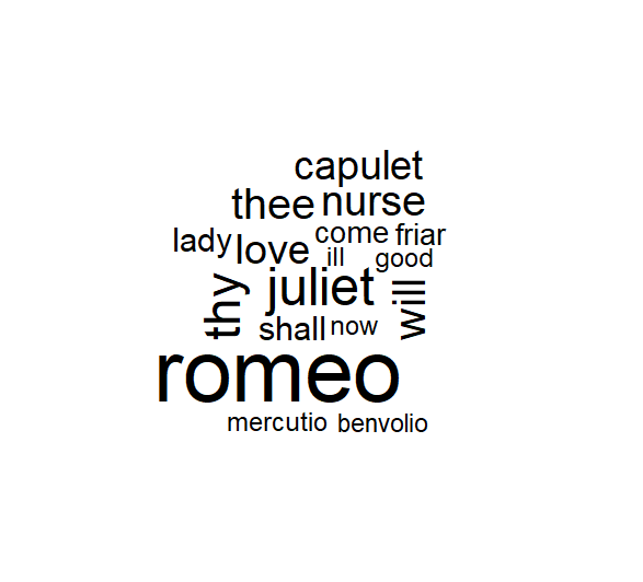
Additional Steps:
Additional wordcloud functions. We can also set the scale of the wordcloud using the scale function. Where 'colors =' we can set the color palette that is used in the wordcloud as well.
##Plots the minimum number (frequency) of words in color
set.seed(142)
wordcloud(names(freq), freq, min.freq=75, scale=c(5, .1), colors=brewer.pal(6, "Dark2")) 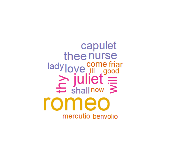
Congratulations you have made your first wordcloud visualization using the tm and wordcloud packages in R.
Additional Steps: Creating a Barplot
We can also create a bar plot that will show the frequency of the words used.
Step 1: Create a TermDocumentMatrix.
## Calculate the rowSums: term_frequency ##################################################################
# Create a TDM from clean_corp: trump_tdm
tdm<-TermDocumentMatrix(docs)
# Convert trump_tdm to a matrix: trump_m
tdm<-as.matrix(tdm)
Step 2: Sum the frequency of words by the rows in the matrix.
We are also going to sort our words in decreasing order by frequency.
term_frequency<-rowSums(tdm)

# Sort term_frequency in descending order
term_frequency<-sort(term_frequency,decreasing=TRU
Step 3: Take a look at the top 10 words.
You can change the number of words to look at by changing [1:10] to any combination of numbers you can think of.
# View the top 10 most common words
term_frequency[1:10]
Result:
romeo juliet thy will nurse thee love capulet shall lady
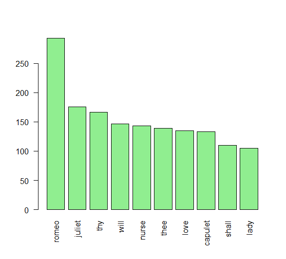
293 176 167 147 143 139 135 133 110 105 Step 4: Plot the barchart.
Again, you can change the rank of the words from the top 1-10 to 5-10 or any combination by changing the [1:10] argument in our code. The las argument allows us to keep the words in a vertical rather than horizontal position when creating our bar chart.
# Plot a barchart of the 10 most common words
barplot(term_frequency[1:10],col="lightgreen",las=2)