Detroit Dataset Description
Type in the variable search term below:
| Variable | Scale | Predictor/Output | Measurement | |
|---|---|---|---|---|
| FTP(Full-Time Police) | Predict future homicides | Predictor | Quantitative | |
| UEMP(Unemployment) | 3.2%-11% | Predictor/Output | Quantitative | |
| LIC(Hangun Licences) | 156.4-1134.2 | Predictor | Quantitative | |
| GR(Handgun Registrations) | 180.5-1029.8 | Predictor/Output | Quantitative | |
| CLEAR(Homicides cleared) | 58.90-94.40 | Predictor/Output | Quantitative | |
| WM(White Males) | 359647-558724 | Predictor/Output | Quantitative | |
| NMAN(Non-manufacturing workers) | 539.1-819.8 | Predictor/Output | Quantitative | |
| GOV(# of government workers) | 133.9-230.9 | Predictor/Output | Quantitative | |
| HE(Average Hourly Earnings) | 2.91-5.76 | Predictor/Output | Quantitative | |
| WE(Average Weekly Earnings) | 117.2-258.1 | Predictor/Output | Quantitative | |
| HOM(# of homicides) | 8.52-52.33 | Predictor/Output | Quantitative | |
| ACC(Death rate in accidents) | 39.17 | Predictor/Output | Quantitative | |
| ASR(# of assaults) | 218-473 | Predictor/Output | Quantitative |
Methods of Analysis
Overview: For the Detroit dataset I have used several modeling techniques (Correlation, Simple Linear Regression, Multiple Linear Regression, Subset Selection, and Generalized Additive Models). The utilization of the plot function helped to determine what variables in the dataset would be significant and those which would not be significant. The correlation function was also used to determine which variables had a high correlation with the outcome variable of homicide. The models were chosen due to the continuous quantitative features of the Detroit dataset. Simple linear regression was utilized and helped to determine the number of predictors in the dataset that would be needed to predict homicide(s) in Detroit . GLM, LDA, QDA, and K-Nearest-Neighbors(KNN) were ignored due to the dataset having continuous variables which would not model well as low or high classification. Lastly the outcome variable is continuous and the above methods are utilized on qualitative outcome variables.
Correlation
Type in the variable search term below:
| Model | Learning Technique | Variables Used | Correlation: Scale = -1 to 1 |
|---|---|---|---|
| Model 1 | Correlation | HOM - FTP | 0.964 |
| Model 2 | Correlation | HOM - UEMP | 0.210 |
| Model 3 | Correlation | HOM - MAN | 0.546 |
| Model 4 | Correlation | HOM - LIC | 0.726 |
| Model 5 | Correlation | HOM - GR | 0.816 |
| Model 6 | Correlation | HOM - CLEAR | -0.968 |
| Model 7 | Correlation | HOM - WM | -0.952 |
| Model 8 | Correlation | HOM - NMAN | 0.955 |
| Model 9 | Correlation | HOM - GOV | 0.958 |
| Model 10 | Correlation | HOM - HE | 0.913 |
| Model 11 | Correlation | HOM - WE | 0.888 |
| Model 12 | Correlation | HOM - ACC | -0.204 |
| Model 13 | Correlation | HOM - ASR | 0.824 |
Best Model Correlation = Model 1- HOM~FTP. The correlation of 0.964 is the best predictor of correlation between homicide and all of the other predictors.
Simple Linear Regression
| Model | Learning Technique | Variables Used | Multiple R-Squared | Adjusted R-Squared |
|---|---|---|---|---|
| Model 14 | Simple Linear Regression | HOM - FTP | 0.93 | 0.923 |
| Model 15 | Simple Linear Regression | HOM - UEMP | 0.04 | -0.04 |
| Model 16 | Simple Linear Regression | HOM - MAN | 0.30 | 0.23 |
| Model 17 | Simple Linear Regression | HOM - LIC | 0.53 | 0.48 |
| Model 18 | Simple Linear Regression | HOM - GR | 0.67 | 0.636 |
| Model 19 | Simple Linear Regression | HOM - CLEAR | 0.94 | 0.93 |
| Model 20 | Simple Linear Regression | HOM - WM | 0.91 | 0.89 |
| Model 21 | Simple Linear Regression | HOM - NMAN | 0.91 | 0.91 |
| Model 22 | Simple Linear Regression | HOM - GOV | 0.92 | 0.91 |
| Model 23 | Simple Linear Regression | HOM - HE | 0.83 | 0.81 |
| Model 24 | Simple Linear Regression | HOM - WE | 0.79 | 0.76 |
| Model 25 | Simple Linear Regression | HOM - ACC | 0.04 | -0.04 |
| Model 26 | Simple Linear Regression | HOM - ASR | 0.68 | 0.65 |
Best Model Simple Linear Regression: The best model is Model 19 and has an adjusted r-squared of 0.93.
summary(lm.fitdetroit6)

Call:
lm(formula = HOM ~ CLEAR, data = Detroit_Data_Ben_Gonzalez)

Residuals:
   Min     1Q Median     3Q    Max
-7.385 -1.636 -1.059  2.804  8.737

Coefficients:
             Estimate Std. Error t value Pr(>|t|)
(Intercept) 127.22163    8.00767   15.89 6.21e-09 ***
CLEAR        -1.25352    0.09724  -12.89 5.55e-08 ***
---
Signif. codes:  0 ‘***’ 0.001 ‘**’ 0.01 ‘*’ 0.05 ‘.’ 0.1 ‘ ’ 1

Residual standard error: 4.264 on 11 degrees of freedom
Multiple R-squared:  0.9379,	Adjusted R-squared:  0.9323
F-statistic: 166.2 on 1 and 11 DF,  p-value: 5.553e-08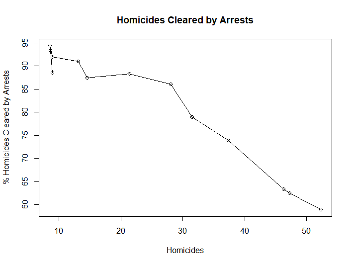
Multiple Linear Regression Table - Detroit Dataset
Type in the variable search term below:
| Model | Learning Technique | Variables Used | Multiple R-Squared | Adjusted R-Squared | p-value |
|---|---|---|---|---|---|
| Model 27 | Multiple Linear Regression | Outcome=HOM Predictors=FTP, MAN, LIC, GR,WM,NMAN,GOV,HE,WE,ASR | 0.998 | 0.9986 | 0.001188 |
| Model 28 | Multiple Linear Regression | Outcome=HOM Predictors=NMAN, GOV, HE, WE, ACC, ASR | 0.9912 | 0.9823 | 6.829E-06 |
| Model 29 | Multiple Linear Regression | Outcome=HOM Predictors=LIC,FTP, GR,HE,WE,NMAN, ASR | 0.9936 | 0.9847 | 3.512E-05 |
Call:
lm(formula = HOM ~ FTP + MAN + LIC + GR + WM + NMAN + GOV + HE +
    WE + ASR, data = Detroit_Data_Ben_Gonzalez)

Residuals:
        1         2         3         4         5         6         7         8         9        10        11
 0.134676 -0.119242  0.035018  0.156071 -0.527640  0.528712 -0.262829  0.140073 -0.115613 -0.167151  0.101167
       12        13
-0.002143  0.098901

Coefficients:
              Estimate Std. Error t value Pr(>|t|)
(Intercept) -2.021e+02  4.986e+01  -4.054   0.0558 .
FTP          2.933e-02  2.345e-02   1.251   0.3375
MAN         -1.150e-01  1.832e-02  -6.279   0.0244 *
LIC          2.704e-02  4.221e-03   6.406   0.0235 *
GR          -4.355e-03  2.362e-03  -1.844   0.2066
WM           2.385e-04  6.509e-05   3.664   0.0671 .
NMAN         1.147e-01  3.824e-02   3.000   0.0954 .
GOV          2.740e-01  9.392e-02   2.917   0.1001
HE          -9.155e+00  3.038e+00  -3.013   0.0947 .
WE           4.393e-01  7.687e-02   5.714   0.0293 *
ASR         -1.437e-02  1.602e-02  -0.897   0.4644
---
Signif. codes:  0 ‘***’ 0.001 ‘**’ 0.01 ‘*’ 0.05 ‘.’ 0.1 ‘ ’ 1

Residual standard error: 0.6188 on 2 degrees of freedom
Multiple R-squared:  0.9998,	Adjusted R-squared:  0.9986
F-statistic: 841.1 on 10 and 2 DF,  p-value: 0.001188
Subset Selection Models
Type in the variable search term below:
| Model | Learning Technique | Variables Used | R.S.Q | Adjusted R2 | Min B.I.C. |
|---|---|---|---|---|---|
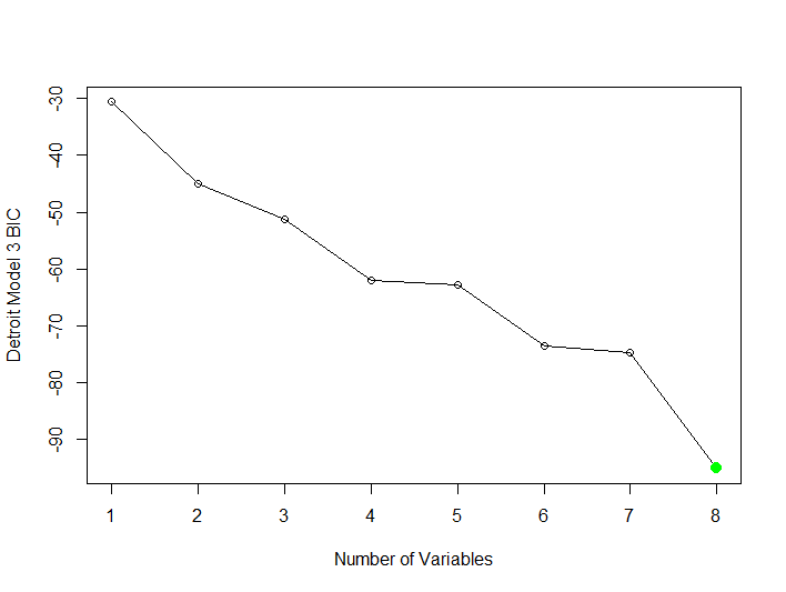
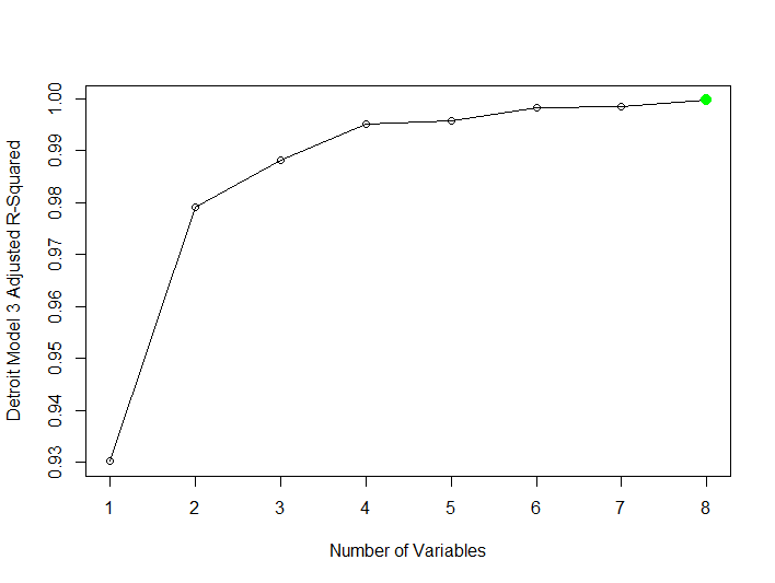
| Model 30 | Subset Model Selection Method=Forward | Outcome=HOM Predictors=All Other Variables | 0.999 | 0.9989 | 8 |
| Model 31 | Subset Model Selection NVMAX=12 | Outcome=HOM Predictors=All Other Variables | 1.000 | 0.9999 | 12 |
| Model 32 | Subset Model Selection Method=Backward | Outcome=HOM Predictors=All Other Variables | 0.999 | 0.999 | 8 |
Best Model Subset Selection: The best subset model selection is Model 32 utilizing the backward method. The model utilizes the lowest BIC and has the highest adjusted r-squared 0.999 utilizing the least number of variables.
Generalized Additive Models
Type in the variable search term below:
| Model | Learning Technique | Variables Used | Total Predictors | Multiple R2 | Adjusted R2 | |
|---|---|---|---|---|---|---|
| Model 33 | Generalized Additive Model Splines Regression | Outcome=HOM Predictors=UEMP,LIC,WE,HE,ASR,NMAN,MAN,ASR | 8 | 0.998 | 0.996 | 6.714e-07 |
| Model 34 | Generalized Additive Model Splines Regression | Outcome=HOM Predictors=MAN,LIC,WM,NMAN,HE,WE | 6 | 0.997 | 0.994 | 2.056e-07 |
| Model 35 | Generalized Additive Model Splines Regression | Outcome=HOM Predictors=FTP,LIC,GR,NMAN,GOV,HE,WE,ASR | 8 | 0.994 | 0.984 | 0.002583 |
| Model 36 | Generalized Additive Model Polynomial Regression | Outcome=HOM Predictors=FTP,LIC,NMAN,GOV^2,HE^3,WE,ASR | 7 | 0.999 | 0.9944 | 0.004688 |
| Model 37 | Generalized Additive Model Polynomial Regression | Outcome=HOM Predictors=FTP^2,GR,LIC^2,NMAN,GOV,HE,WE,ASR | 8 | 0.998 | 0.993 | 0.005753 |
Best Model Generalized Additive Model: The best model for the generalized additive model is Model 36 that utilizes polynomial regression. The model utilizes the least amount of predictors of all the generalized additive models. The model has the highest adjusted r-squared of 0.9944 that utilizes the least number of predictors. The p-values is also low at 0.004688.
Analysis of Variance Table

Response: HOM
             Df  Sum Sq Mean Sq   F value    Pr(>F)
FTP           1 2994.37 2994.37 1978.9471 0.0005049 ***
LIC           1  151.19  151.19   99.9199 0.0098602 **
NMAN          1   30.18   30.18   19.9431 0.0466611 *
poly(GOV, 2)  2   18.27    9.13    6.0363 0.1421203
poly(HE, 3)   3   23.30    7.77    5.1325 0.1673830
WE            1    0.65    0.65    0.4326 0.5782914
ASR           1    0.80    0.80    0.5300 0.5423085
Residuals     2    3.03    1.51
---
Signif. codes:  0 ‘***’ 0.001 ‘**’ 0.01 ‘*’ 0.05 ‘.’ 0.1 ‘ ’ 1
> summary(gam.detroitmodel44)

Call:
lm(formula = HOM ~ FTP + LIC + NMAN + poly(GOV, 2) + poly(HE,
    3) + WE + ASR, data = Detroit_Data_Ben_Gonzalez)

Residuals:
        1         2         3         4         5         6         7         8         9        10        11        12
 0.008567 -0.163223  0.199979 -0.520727  0.990593 -0.700423  0.534176 -0.012935 -0.837255  0.361341  0.277549 -0.149193
       13
 0.011550

Coefficients:
               Estimate Std. Error t value Pr(>|t|)
(Intercept)   -70.16794  127.52402  -0.550    0.637
FTP            -0.29850    0.31798  -0.939    0.447
LIC             0.03193    0.01821   1.753    0.222
NMAN            0.12534    0.18927   0.662    0.576
poly(GOV, 2)1   1.33967   48.34475   0.028    0.980
poly(GOV, 2)2  40.96870   38.86995   1.054    0.402
poly(HE, 3)1  -42.82354   75.21346  -0.569    0.627
poly(HE, 3)2   -3.68839   10.90049  -0.338    0.767
poly(HE, 3)3   -3.24754    7.03880  -0.461    0.690
WE              0.54739    0.55821   0.981    0.430
ASR            -0.02719    0.03734  -0.728    0.542

Residual standard error: 1.23 on 2 degrees of freedom
Multiple R-squared:  0.9991,	Adjusted R-squared:  0.9944
F-statistic: 212.7 on 10 and 2 DF,  p-value: 0.004688
> summary(gam.detroitmodel44)
Call:
lm(formula = HOM ~ FTP + LIC + NMAN + poly(GOV, 2) + poly(HE,
3) + WE + ASR, data = Detroit_Data_Ben_Gonzalez)
Residuals:
1 2 3 4 5 6 7 8 9 10 11 12
0.008567 -0.163223 0.199979 -0.520727 0.990593 -0.700423 0.534176 -0.012935 -0.837255 0.361341 0.277549 -0.149193
13
0.011550
Coefficients:
Estimate Std. Error t value Pr(>|t|)
(Intercept) -70.16794 127.52402 -0.550 0.637
FTP -0.29850 0.31798 -0.939 0.447
LIC 0.03193 0.01821 1.753 0.222
NMAN 0.12534 0.18927 0.662 0.576
poly(GOV, 2)1 1.33967 48.34475 0.028 0.980
poly(GOV, 2)2 40.96870 38.86995 1.054 0.402
poly(HE, 3)1 -42.82354 75.21346 -0.569 0.627
poly(HE, 3)2 -3.68839 10.90049 -0.338 0.767
poly(HE, 3)3 -3.24754 7.03880 -0.461 0.690
WE 0.54739 0.55821 0.981 0.430
ASR -0.02719 0.03734 -0.728 0.542
Residual standard error: 1.23 on 2 degrees of freedom
Multiple R-squared: 0.9991, Adjusted R-squared: 0.9944
F-statistic: 212.7 on 10 and 2 DF, p-value: 0.004688Tree Based Methods
Type in the variable search term below:
| Model | Learning Technique | Variables Used | Mean of Squared Residuals | Minimum M.S.E. | % Variance Explained | Optimal Configuration | Optimal Trees/Interaction F-Statistic |
|---|---|---|---|---|---|---|---|
| Model 38 | Random Forest | Outcome=HOM Predictors=All other variables | 216.2263 | 212.892 | -8.47 | 7 Predictors | 10 Trees |
| Model 39 | Random Forest K-Fold CV Approach | Outcome=HOM Predictors=All other variables | 216.2263 | 5.84121 | -8.47 | 8 Predictors | 3 Trees |
| Model 40 | Random Forest Boosting K-Fold CV Approach | Outcome=HOM Predictors=All other variables | N/A | N/A | N/A | N/A | N/A |
| Model 41 | Linear Model K-Fold CV Approach | Outcome=HOM Predictors=All other variables | N/A | 210.021 | N/A | 4 Predictors | 9 Trees |
Note: N/A = Sample Size too small to utilize method
Best Model Tree Based Methods: The best model of the tree based methods is Model 41 the Linear Model K-Fold CV Approach Model. While it has a higher minimum MSE. The other models have a negative percentage of the variance explained for the data. The optimal number of predictors is 4 and the optimal number of trees is 9.
Validation Set Approach
Type in the variable search term below:
| Model | Learning Technique | Variables Used | Minimum M.S.E. |
|---|---|---|---|
| Model 42 | Cross Validation Approach | Outcome=HOM Predictor=LIC | 180.6076 |
| Model 43 | K-Fold Cross Validation | Outcome=HOM Predictor=LIC | 108.0558 |
| Model 44 | K-Fold Cross Validation | Outcome=HOM Predictor=LIC | 179.4411 |
Best Model Validation Set Approach: The best model for the validation set approach is Model 43. The K-Fold Cross Validation Approach has the lowest MSE 108.0558 out of all of the models in the set.
> cv.error

[1]  182.3850  108.0558  592.6336  519.8474 1318.5811
Results: Best Model Selection - Detorit Dataset
Type in the variable search term below:
| Model | Learning Technique | Variables Used | Correlation(s)/MSE/RSQ/Adjusted R2/%Variance Explained | AIC/BIC/CP | Optimal Configuration/F-Statistic/p-value |
|---|---|---|---|---|---|
| Model 1 | Simple Linear Regression | Outcome=HOM Predictor=FTP | Correlation=0.964 | ||
| Model 2 | Multiple Linear Regression | Outcome=HOM Predictors=FTP, MAN, LIC, GR,WM,NMAN,GOV,HE,WE,ASR | Multiple R-Squared=0.9998 ADJR2=0.9986 | p-value=0.001188 | |
| Model 3 | Subset Selection Method=Backward | Outcome=HOM Predictors=All Other Variables | Multiple R-Squared=0.999 ADJR2=0.999 | BIC = 8 | |
| Model 4 | Generalized Additive Model / Polynomial Regression | Outcome=HOM Predictors=FTP,LIC,NMAN,GOV^2,HE^3,WE,ASR | Multiple R-Squared=0.999 ADJR2=0.9944 | p-value=0.004688 | |
| Model 5 | Tree Based Methods Linear Model K-Fold CV Approach | Outcome=HOM Predictors=All other variables | Optimal Configuration= 4 Predictors 9 Trees | ||
| Model 6 | Validation Set Approach | Outcome=HOM Predictor=LIC | MSE = 108.0558 |
> anova(gam.detroitmodel44)

Analysis of Variance Table

Response: HOM
             Df  Sum Sq Mean Sq   F value    Pr(>F)
FTP           1 2994.37 2994.37 1978.9471 0.0005049 ***
LIC           1  151.19  151.19   99.9199 0.0098602 **
NMAN          1   30.18   30.18   19.9431 0.0466611 *
poly(GOV, 2)  2   18.27    9.13    6.0363 0.1421203
poly(HE, 3)   3   23.30    7.77    5.1325 0.1673830
WE            1    0.65    0.65    0.4326 0.5782914
ASR           1    0.80    0.80    0.5300 0.5423085
Residuals     2    3.03    1.51
---
Signif. codes:  0 ‘***’ 0.001 ‘**’ 0.01 ‘*’ 0.05 ‘.’ 0.1 ‘ ’ 1
summary(gam.detroitmodel44)
Call:
lm(formula = HOM ~ FTP + LIC + NMAN + poly(GOV, 2) + poly(HE,
3) + WE + ASR, data = Detroit_Data_Ben_Gonzalez)
Residuals:
1 2 3 4 5 6 7 8 9 10 11 12
0.008567 -0.163223 0.199979 -0.520727 0.990593 -0.700423 0.534176 -0.012935 -0.837255 0.361341 0.277549 -0.149193
13
0.011550
Coefficients:
Estimate Std. Error t value Pr(>|t|)
(Intercept) -70.16794 127.52402 -0.550 0.637
FTP -0.29850 0.31798 -0.939 0.447
LIC 0.03193 0.01821 1.753 0.222
NMAN 0.12534 0.18927 0.662 0.576
poly(GOV, 2)1 1.33967 48.34475 0.028 0.980
poly(GOV, 2)2 40.96870 38.86995 1.054 0.402
poly(HE, 3)1 -42.82354 75.21346 -0.569 0.627
poly(HE, 3)2 -3.68839 10.90049 -0.338 0.767
poly(HE, 3)3 -3.24754 7.03880 -0.461 0.690
WE 0.54739 0.55821 0.981 0.430
ASR -0.02719 0.03734 -0.728 0.542
Residual standard error: 1.23 on 2 degrees of freedom
Multiple R-squared: 0.9991, Adjusted R-squared: 0.9944
F-statistic: 212.7 on 10 and 2 DF, p-value: 0.004688Best Model Selection: The best model for the Detroit Dataset is Model 4 in the best model selection table. The learning technique is the generalized additive model-polynomial regression. This model has the highest adjusted r-squared utilizing the least amount of predictors at 7. The p-value is 0.004688 and is the lowest for this number of predictors. The significant predictors for the outcome variable are FTP(full time police), LIC( Gun Licenses), and NMAN(Non-Manufacturing Jobs).